
There are various Quantity Theory of Money which have been put forward for explaining the determination of the value of money. Jean Bodin presented the quantity theory of money in 1568 for the first time. Afterward, John Law, David Hume, Henry Thornton, David Ricardo, J.S. Mill and Simmon Newcomb have also worked on this theory.

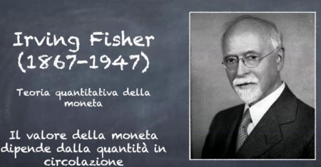
But it was popularized by professor Irving Fisher with the help of an equation in his book “Purchasing Power of Money” in 1911 A.D. This theory is based on medium of exchange function of money. Monetary policy is the basis of ups and down in value of money and price level. Here, we explain the following important theories of QTM:
3 Best Quantity Theory of Money With Examples;If You Are Student of Money And Finance.
- Quantity Theory of Money – Transaction Approach.
- Cash Balance Quantity Theory of Money.
- Modem Quantity Theory of Money.
Classical quantity theory qf money;(FISHER’S TRANSACTION APPROACH)
According to this theory, the value of money is dependent on the quantity of money in circulation. Any change in the total quantity of money in the country affects prices and the change in prices of goods affects the value of money.
In simple words, quantity theory of money states that changes in general price level occur due to changes in quantity of money in circulation, i.e.l an increase in quantity of money raises the price level or a contraction in the quantity of money will lead to fall in general price level,
According to Irvirig Fisher:
“Other things remaining unchanged, as the quantity of money in circulation increases, the price level also increases in direct proportion and the value of money decreases and vice versa”.
According to F.W. Taussig:
“Double the quantity of money and other things being equal, price will be twice as high as before, and me value of money one half Half the quantity of money and other things being equal, prices will be half of what they were before and the value of money double”.
EXPLANATION:
Thus we see that according to the above given definitions, the change in quantity of money affects the price level in direct proportion and since value of money and price level have inverse relation with each other, we can say that quantity of money and value of money is inversely proportional. .t
Equation of Exchange:
Prof. Irving Fisher has expressed the quantity theory of money in a simple equation, which is called equation of exchange. It is as:
Where P = General price level.
M = Quantity of money or stock of money.
V = Velocity of money in circulation.
T = Volume of transactions i.e. number of goods to be bought and sold through money.
M’ – Credit money.
V’ = Velocity of credit money
In this formula (MV + M’V’) represents supply of money and demand for money equals to supply of money. Prof. Fisher assumes that in short period T and V remain constant. Therefore P will change directly with M. Example:
Suppose the initial position of the economy is as:
M
I
P
= 300
= 2
= 40
MV + M’V
M’ =100
V’ =2
By putting the values in equation:
P
300 x 2+ 100×2
40 — Rs*
Now to see the effect of change in quantity of money over price and value of money, let double the M, keeping velocity (V) and quantity of goods as constant.
P
600×2 + 200×2
= Rs. 40
Thus we see that when M is doubled, price level is also doubled which means that value of money has fallen to one half.
Now, we half the M:
P
150 x 2 + 50x 2 „ _
4Q —Rs- 10
Thus we see that if we half the M, the price will also be half and value of money will be doubled.
Quantity theory of money can be explained with the help of following diagrams:
Quantity of money
When quantity of money is Qi, price is P| and when quantity of money rises to Q2, means double, price also increases to P2 and so on. It means there is direct relationship between the quantity of money and price.
ASSUMPTIONS of Classical quantity theory qf money
The quantity theory is based on following assumptions.
- Full Employment:
The theory is based on the assumption of full employment in the economy.
- Price Level is a Passive Factor:
The theory assumes that price level (P) is affected by other factors of equation but it does not affect them.
- Constant Velocity of Money:
In Fisher’s equation, the velocity of circulation of money (v) and bank money (v’) are assumed to be constant.
- Constant Volume of Trade:
The total volume of transactions (T) remains unaffected by changes in M and M’.
- Barter Transaction:
Barter means exchange of goods and services for goods and services without the use of money. The barter dealing can be excluded altogether while dealing with quantity theory.
- Long Period:
The theory applies to the changes in prices only in long period, because quantity of money does not affect price level and value of money in short run.
- Constant relation between M and M’:
In Fisher’s equation, it is assumed a proportional relationship between currency money (M) and bank money (M’).
CRITICISM of Classical quantity theory qf money
This theory has been criticized on the following grounds:
- Useless Assumptions:
This theory is based on certain assumptions ‘‘other things remaining the same ” which are not always true. Therefore, theory is not correct.
- Dependent Variables:
All the assumptions are inter-linked. If one variable is changed the other is also changed. Therefore, this theory is not correct.
- Circulation of Money:
It is very difficult to measure the circulation of money in the country; therefore, velocity cannot be calculated within the country.
- Dynamic Theory:
It is a dynamic theory, which is not constant. Therefore, the value of money is not exactly measurable.
- Supply Side:
This theory is one sided because the quantity of money can be doubled but it is not possible to half the quantity of money.
- Proportionate Change:
According to Fisher, the increase or decrease in the quantity of money brings proportionate change in the price level while the history shows that it is not true
- Trade Cycle:
According to this theory government can increase the quantity of money to remove the deflation and decrease the supply of money to control inflation. But in 1930, when great depression took place, every country tried his best to increase the quantity of money but the prices did not rise and depression could not be removed.
- Ignores the Rate of Interest:
Another serious defect is that this theory does not take into consideration the influences of the rate of interest of cash balances.
Quantity Theory of Money With Examples And Critisim
2.CASH BALANCE QUANTITY THEORY OF MONEY
Cambridge economists Marshall, Pigou, Robertson and Keynes formulated the cash balance approach to analyze the value of money known as Cambridge Cash Balances approach. The Cash Balances version of the quantity theory of money considers both supply of and demand for money as the determinants of the value of money.
According to The Theory:
“ Value of money depends upon the demand and supply of money. The value of money is fixed at the point where demand for money and supply of money is equal”.
Supply of Money:
Supply of money is the quantity of legal tender money and its velocity and quantity of bank money and its velocity. According to Cambridge economists, supply of money over a short period does remain constant. So determination of value of money largely depends upon the demand for money.
Demand for Money:
Demand for money is the desire of people to hold cash balances for transaction, precautionary and speculation motives. In other words, demand for money means the proportion of total income, which people hold in form of cash, for the abovementioned purposes.
CAMBRIDGE EQUATIONS
The Cambridge economists explained their approaches inform of equations known as cash-balance equations of exchange or Cambridge equations of exchange, which are as under.
- Marshairs Equation:
Allred Marshall in his bock “Money Credit and Commerce” expressed his ideas regarding the value of money. One of his students and very well known economist “M. Friedman” presented the views of his teacher algebraically in “Quarterly Journal of Economics” in the following shape.
M = KPY (or) P = £7
Where: P = The general price level ।
M = Money supply
K = Demand for money (portion of income held in form of cash)
Y = Aggregate real income
Keeping K and Y constant in equation, we find:
M = P
The equation shows a direct and proportionate relationship between price level and quantity of money.
- Pigou’s Equation:
Pigou started his career, as a follower of neoclassical views of Marshall and remained loyal to neoclassical. He was the first Cambridge economist who presented the theory regarding value of money algebraically in his article “The Value of Money” appeared in the Quarterly Journal of Economics in November 1917.
p = r M
Where: P = Purchasing power of money
K = Demand for money
R = Total real resources (Agricultural output)
M = Quantity of money (Legal tender money)
Keeping K and R constant we get:
The equation shows inverse and proportionate relation between price level and quantity of money.
- Robertson’s Equation:
If we take P as price level instead of the value of money as it was in Pigou’s equation then Robertson’s equation exactly resembles Pigou’s equation.
‘ P = MKT
Where: P = General price level ‘
K = Demand for money
M = Quantity of money
T = Total output
Keeping K and T constant, we get the same direct and proportionate relation between the price level and quantity of money.
- Keynesian’s Equation:
Keynes started his career as follower of neoclassical views of Marshall but he did not remain loyal to neoclassical. He laid down the base of modem economics and became the founder of modem macroeconomics. According to Keynes, people hold money for transaction, precautionary and speculation motives. Further, he measures the demand for money in terms of consumption units and a consumption unit is a basket of standard articles of consumption.
N
N = PK (or) P = v
- K
Where: P = General price level (The price of a consumption unit)
N = Total currency in circulation
K = Number of consumption units in the form of cash
Subsequently, Keynes modified his equation to incorporate the bank deposits.
N = P(K + RK’)
Where: R = Cash reserve ratio of banks
K = Number of consumption units in form of cash
K’ = Number of consumption units in form of bank deposits
By keeping K, R and K’ constant:
N = P
The equation shows a direct and proportionate relation between quantity of money and price level.
CRITICISM of CASH BALANCE QUANTITY THEORY OF MONEY
- Ignored Rate of Interest:
The theory ignores the influences, of rate of interest. Theory states that price level varies directly and the value of money inversely to any change in quantity of money. But, the rate of interest also exerts a decisive and significant influence upon the price level.
- Illogical Assumption:
Theory assumes the factors K, Y, T, R as constant, which is illogical. It is not essential that the cash balances and the income level of people should remain constant even in short run.
- Truism:
The cash balances equations are also truisms like transaction equation of Fisher. So, it is considered as old wine in a new bottle.
- No Proper Explanation:
Theory in unable to explain the changes in price level due to changes in the proportions of deposits which are held for income, business and savings purposes.
- Variation in Price Level:
The cash balances theory ignores financial and industrial transactions. It is also failed to explain the variations in price level due to inequality of savings and investment in the economy.
6.Same Mistake:
Cambridge economists criticized the Irving Fisher’s equation as it establishes a proportionate and direct relation between price level and quantity of money but the Cambridge economists committed the same mistake.
- Money and Commodity Market:
It is pointed out that the cash balances equations laid undue concentration on money market and ignored commodity market. In this theory, Cambridge economists failed to integrate the commodity market and the money market.
MODERN QUANTITY THEORY QF MONEY By Milton Friedman
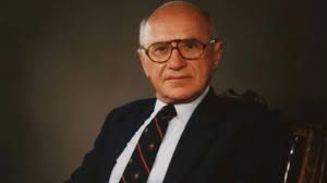
Modem quantity theory of money was presented by Milton Friedman in his article “The Quantity Theory of Money – A Restatement” published in 1956. Friedman regards money in terms of other theory of consumer choice.
Money is a type of durable consumer good and people demand it for the services it performs and it is demanded as an asset or capital.
In Friedman’s view the assets or wealth can be held in form of money, bonds, shares, goods and human capital. Demand for money depends upon the volume of total wealth and the relative return on different forms of assets which can be held as wealth. It means this quantity theory of money is just a theory of demand for money and not the theory of income, investment and employment.
[DETERMINANTS OF DEMAND FOR MONEY]
According to Milton Friedman, the demand for money or an asset is the function of the following factors.
- Return on Bonds:
If the rate of return on the bonds is higher in the market, the demand for money shall be smaller and vice versa.
- Return on Shares:
If the rate of return on shares is higher then people will prefer to keep their wealth in form of shares which decreases the demand for money and vice versa.
- Change in Prices:
If the prices are rising rapidly in a country, the demand for money shall be smaller and the people hold smaller amount of money to avoid a fall in the real purchasing power of the money.
- Degree of Risk:
The degree of risk about the return on an asset also affects the demand for assets. If the risk increases on an asset then its demand falls and demand for other alternative assets increases.
- Liquidity:
Liquidity means that how quickly an asset can be converted into cash. Keeping all other things constant, if the liquidity of an asset is higher then its demand will also be higher and vice versa.
EQUATION OF DEMAND FOR MONEY:
Based upon the factors discussed above, Milton Friedman developed the following equation of demand for money.
Md = f(U, P, Y, I, P*)
Here: Md = Demand for money
U = Utility of money
Y = Level of income
P = Price level
I = Rate of interest
P* = Inflation rate
Milton Friedman said that the utility of money normally remains same and he did not observe a severe type of inflation, which could influence the demand for money. So he deleted U and P* from his demand for money.
Md = f(P, Y, I)
BASIC FEATURES OF THE THEORY
- The demand for money is influenced by the change in the level of income and the relation between demand for money and level of income is non-proportional.
- The demand for money is influenced by the change in price level and there is a proportional relationship between price level and demand for money. According to Friedman’s analyses, 1% increase in price level also leads to 1% increase in demand for money.
- The demand for money is influenced by change in the rate of interest and there is inverse relation between rate of interest and demand for money. If rate of interest increases the demand for money falls and vice versa.
- Money market is in equilibrium when “Md = Ms”.
If there is a change in a supply of money then Y, P and I also change and ultimately demand for money changes and eventually Ms becomes equal to Md.
CRITICISM of QUANTITY THEORY QF MONEY By Milton Friedman
Milton Friedman theory has been criticized on the following grounds:
- Money Supply and Money GNP:
According to Friedman, there is a positive relationship between money supply and money GNP but in actual there is no correlation between them due to number of variables which cannot be controlled.
- Proportional Relationship:
Friedman observed proportional and direct relationship between price and demand for money but in actual it does not happen. The fact is that the demand for money is more than proportionately to change in the income level.
3.Money is not Actually Goods:
If the income of a person increases, he increases his expenses on luxury goods. Since money is considered as a good by Friedman and according to his observation demand for luxury goods increases when the income of people in USA increases. Hence he treated money as luxury good but no such effects have been found in England.
- Certain Variables Ignored:
He ignored certain variables like price, output and rate of interest which may effect the supply of money.
- Wealth as Variable:
Friedman presented his revised demand function in 1982 in which he included wealth as variable alongwith income. According to him both the variables affect the demand for money. But it was criticized because income is a form of wealth and when income has been discussed earlier then there was no need to discuss wealth separately.